Making reproducible documents with R
Session details
- Date of session: 09 Nov, 2018
- Instructor: Luke Johnston
- Contributions from: Maria Izabel Cavassim Alves (@izabelcavassim)
- Session level: Beginner
- Part of the “Beginner Series”
Required packages to install:
Objectives
- To become aware of the importance of reproducibility of data analyses.
- To learn how to generate high quality reports that can be shared with a broader audience.
- To create reproducible documents interwoven with R code that can be run on updated or different data sets.
- To use Rstudio not as a data science tool but also as a text editor and compiler!
- To know where to go for continued learning.
At the end of this session you will be able:
- Create a new RMarkdown document.
- Write text, headers, citations, and other report writing tasks in Markdown.
- Insert R code chunks that will create figures, tables, or numbers.
- Generate an analytically reproducible Word or HTML document.
Resources for learning and help
For learning:
- RStudio tutorial on using RMarkdown
- Markdown syntax guide
- Online book for RMarkdown
- R for Data Science
For help:
- RStudio helpful cheatsheets
- R Markdown cheatsheet (downloads a pdf file)
- R Markdown reference cheatsheet
Why try to be reproducible?
Well, first thing, reproducibility and replicability is a cornerstone of doing science. However, the current concept of reproducibility relates more to computational reproducibility: Hypothetically, if you gave someone your data, your code, and your paper, would they be able to generate the exact same numbers you report in your manuscript and in your tables and figures? Research shows that this is not at all the case… even when the same researcher tries to reproducible their own paper!
Being reproducible and writing a reproducible document/manuscript does several things for you:
- Makes your science better.
- Makes you more efficient and productive, since less time is spent between coding and putting your results in the document.
- Makes you more confident in your results, since what you report is what you actually got from the analysis.
- Its actually a lot of fun! ;)
Let’s get to learning about R Markdown!
Markdown syntax
Headers
Such as for a section, subsection, subsubsection, etc.
# Header 1gives…
Header 1
## Header 2gives…
Header 2
### Header 3gives…
Header 3
Text formatting
**bold**gives bold.*italics*gives italics.super^script^gives superscript.sub~script~gives subscript.
Lists
Unnumbered list:
- item 1
- item 2
- item 3
gives…
- item 1
- item 2
- item 3
Numbered list:
1. item 1
2. item 2
3. item 3
gives…
- item 1
- item 2
- item 3
Block quotes
One can also create quotes:
> Block quotegives…
Block quote
Exercise: Construct an outline for a (hypthetical) paper
Time: 10 min
Open RStudio and create an R Markdown document:
File -> New File -> R Markdown
Save the file and call the file exercise.Rmd. In the R Markdown document, include the following “Header 1” # sections:
- Abstract
- Introduction
- Material and Methods
- Results
- Discussion
- Conclusion
Compile it by pressing the icon Knit to HTML or by typing Ctrl-Shift-K. Then:
- Write some random words below the Abstract section, while using bold and italics.
- Include an unnumbered list below Introduction listing two or three fake objectives.
- Include a “Header 2” (
##) called “Statistical analysis” below “Material and Methods”.
Compile (“knit”“) the document again and see what happens.
Adding footnotes, pictures, and links to your document
Footnotes can be done using the following command:
Footnote[^1]

[^1]: Footnote content
gives…
Footnote1
A .png .jpeg or .pdf image can be attached in the following way:
gives…

image caption
And a link can be linked in the following format:
[Link](https://google.com)gives…
Exercise: Add more to your Markdown document!
Time: 8 min
Now you are asked to include in your “skecthed article” what we just have learned.
- Include a random picture with caption (of your research or of any .png you find in your PC).
- Include a footnote.
- Include the link of the AUOC webpage (
https://au-oc.github.io) in your document.
The best part! Inserting R code
One of the most powerful and useful features of Rmarkdown, is its ability to combine text and code in the same document! You can insert plots by including a code chunk like below. The options added to the code chunk tell it to add a caption, and set the height and width of the figure.
```{r plot_sepal, fig.cap="Figure title here", fig.height=8, fig.width=8, echo=FALSE}
plot(Sepal.Length ~ Sepal.Width, data = iris)
```
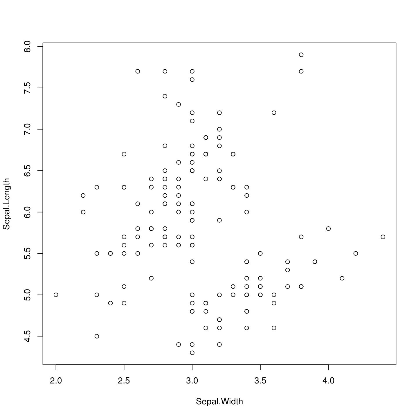
Figure title here
You can also create tables by using the kable() function in the knitr package.
```{r}
knitr::kable(head(iris), caption = "Table caption here")
```
| Sepal.Length | Sepal.Width | Petal.Length | Petal.Width | Species |
|---|---|---|---|---|
| 5.1 | 3.5 | 1.4 | 0.2 | setosa |
| 4.9 | 3.0 | 1.4 | 0.2 | setosa |
| 4.7 | 3.2 | 1.3 | 0.2 | setosa |
| 4.6 | 3.1 | 1.5 | 0.2 | setosa |
| 5.0 | 3.6 | 1.4 | 0.2 | setosa |
| 5.4 | 3.9 | 1.7 | 0.4 | setosa |
The knitr:: part of the code tells R where the kable function comes from. So the :: is telling R “hey, look in the knitr package for the kable function”.
For small and not too complex tables, you can also create it outside of a R chunk using the Markdown syntax:
|               | diverged | polymorphic |
|:------------------:|:--------:|:-----------:|
|   **synonymous**   |   1300   |    2109     |
| **non-synonymous** |   700    |     891     |
gives…
| diverged | polymorphic | |
|---|---|---|
| synonymous | 1300 | 2109 |
| non-synonymous | 700 | 891 |
You can hide the code chunk but keep the output by using the echo=FALSE option:
```{r, echo=FALSE}
cor(iris$Sepal.Length, iris$Sepal.Width)
```
#> [1] -0.1175698Inline R code
You can also include R code within the text. You can use this to directly insert numbers into the text of the document. By using something like:
The mean of the sepal length is
`r round(mean(iris$Sepal.Length), 2)`.Gives…
The mean of the sepal length is 5.84.
Exercise: Add a plot and table to “Results”
Time: 10 min
You now need to create a chunck of code in the Results section. If you have any plot from your own research that you want to create feel free to do it so. Otherwise you can just use the iris data:
Use
names(CO2)to find the names of columns from the CO2 dataset. Choose two columns. Create a code chunk with a captionfig.capoption and thefig.widthof 10 and afig.heightof 6. Include in the code chunk the function, replacing the__with the two columns you chose:- Create a table of the
head()of theCO2dataset using the R functionknitr::kable(). - Create an inline R code that shows the sum of 2 plus 2 (
2 + 2). Try to make a similar table as the one below, but using your own Markdown syntax in your document.
| Weather | Activity |
|---|---|
| Sunny | Beach or biking |
| Snowy | Movies or reading |
Other features
Citing literature with Rmarkdown
If you want to insert a citation use [@Hoejsgaard2006a] to get it to look like: (Højsgaard, Halekoh, and Yan 2006)… the reference is then inserted onto the bottom of the document. You need to add a line to the YAML header like this:
---
title: "My report"
author: "Me!"
bibliography: my_references.bib
---
Making your report prettier
This really only applies to HTML and PDF2 documents. If you want to change the theme, add an option to the YAML header so it looks like:
---
title: "My report"
output:
    html_document:
        theme: sandstone
---
Check out the R Markdown documentation for more types of themes you can use for HTML documents.
Ending remarks
We hope that we’ve shown the power that comes with using R Markdown and that we’ve convinced you enough to try using R Markdown for writing your reports! Believe us, it can save soooo much time in the end after you’ve learned how to incorporate text with R code when writing any type of document that relies on results from data analysis or presentation. R Markdown is a powerful tool for reproducibility and for creating beautiful reports! There are many other amazing features of R Markdown that you can learn about from the resources above. Try it out and learn more about it!
References (add this at end to separate the ref list)
Højsgaard, Søren, Ulrich Halekoh, and Jun Yan. 2006. “The R Package Geepack for Generalized Estimating Equations.” Journal of Statistical Software 15/2:1–11.
This work is licensed under a Creative Commons Attribution 4.0 International License. See the licensing page for more details about copyright information.